
반응형
Notice
Recent Posts
Recent Comments
Link
| 일 | 월 | 화 | 수 | 목 | 금 | 토 |
|---|---|---|---|---|---|---|
| 1 | 2 | 3 | ||||
| 4 | 5 | 6 | 7 | 8 | 9 | 10 |
| 11 | 12 | 13 | 14 | 15 | 16 | 17 |
| 18 | 19 | 20 | 21 | 22 | 23 | 24 |
| 25 | 26 | 27 | 28 | 29 | 30 | 31 |
Tags
- parrec
- 확산강조영상
- MICCAI
- nfiti
- 모수적 모델
- deep learning #segmentation #sementic #pytorch #UNETR #transformer #UNET #3D #3D medical image
- Surgical video analysis
- genetic epidemiology
- monai
- parametric model
- PYTHON
- TabNet
- non-parametric model
- parer review
- words encoding
- MRI
- paper review
- 파이썬
- 유전역학
- 확산텐서영상
- decorater
- TeCNO
- 비모수적 모델
- nlp
- Phase recognition
- 데코레이터
- tabular
- 코드오류
- nibabel
- precision #정밀도 #민감도 #sensitivity #특이도 #specifisity #F1 score #dice score #confusion matrix #recall #PR-AUC #ROC-AUC #PR curve #ROC curve #NPV #PPV
Archives
- Today
- Total
KimbgAI
[ML] Data augmentation for 3D medical image 본문
반응형
augmentation은 적은 데이터를 가지고도 데이터 풍부한 표현을 학습할 수 있는 장점이 있습니다.
그 중에서도 3D augmentation은 일반적인 2D augmentation과는 다른 특징들이 있는데,
이 글에서는 그와 관련된 내용을 담고 있습니다.
monai, TorchIO 등 3D augmentation을 위한 라이브러리들이 몇몇 있지만,
여기서는 monai 기반 augmentation 적용 방법을 소개합니다.
본 내용은 아래 내용을 첨삭하여 작성했습니다.
3d_image_transforms.ipynb
Run, share, and edit Python notebooks
colab.research.google.com
Contents
- 데이터 준비
- 데이터 형태 확인
- 샘플 시각화
1. 채널 첫번째 디멘젼으로 보장하기
2. axis 통일하기
3. voxel size 통일하기
4. random affine 변환 (회전, 확대, 전단 등)
5. random elastic 변환 (울퉁불퉁하게 하기)
Setup environment
import torch

from monai.transforms import (
    EnsureChannelFirstd,
    LoadImage,
    LoadImaged,
    Orientationd,
    Rand3DElasticd,
    RandAffined,
    Spacingd,
)
from monai.config import print_config
from monai.apps import download_and_extract
import numpy as np
import matplotlib.pyplot as plt
import tempfile
import shutil
import os
import glob
데이터 준비
- 데이터가 있으면 data_dir를 자신의 경로에 맞게 수정해주세요.
- 데이터가 없으면 USE_MY_DATA 를 False로 두고 다운로드 받으면 됩니다.
- The dataset comes from http://medicaldecathlon.com/.
USE_MY_DATA = True

if not USE_MY_DATA:
    directory = os.environ.get("MONAI_DATA_DIRECTORY")
    root_dir = tempfile.mkdtemp() if directory is None else directory
    print(f"root dir is: {root_dir}")

    resource = "https://msd-for-monai.s3-us-west-2.amazonaws.com/Task09_Spleen.tar"
    md5 = "410d4a301da4e5b2f6f86ec3ddba524e"

    compressed_file = os.path.join(root_dir, "Task09_Spleen.tar")
    data_dir = os.path.join(root_dir, "Task09_Spleen")
    if not os.path.exists(data_dir):
        download_and_extract(resource, compressed_file, root_dir, md5)

else:
    data_dir = '/data/MSD/Task09_Spleen'
train_images = sorted(
glob.glob(os.path.join(data_dir, "imagesTr", "*.nii.gz")))
train_labels = sorted(
glob.glob(os.path.join(data_dir, "labelsTr", "*.nii.gz")))
data_dicts = [
{"image": image_name, "label": label_name}
for image_name, label_name in zip(train_images, train_labels)
]
train_data_dicts, val_data_dicts = data_dicts[:-9], data_dicts[-9:]
train_data_dicts[0]{'image': '/data/MSD/Task09_Spleen/imagesTr/spleen_10.nii.gz',
'label': '/data/MSD/Task09_Spleen/labelsTr/spleen_10.nii.gz'}
데이터 형태 확인
- monai의 LoadImage 클래스는 nibabel를 통해 이미지를 간편하게 로드해줍니다.
- 기본적으로 image array를 return하지만, affine information이나 voxel size같은 metadata도 출력할 수 있습니다.
loader = LoadImage(dtype=np.float32, image_only=True)
image = loader(train_data_dicts[0]["image"])
print(f"image shape: {image.shape}")
print(f"image dtype: {image.dtype}")
print(f"image affine: {image.meta['affine']}")
print(f"image pixdim: {image.pixdim}")
image shape: (512, 512, 55)
image dtype: torch.float32
image affine: tensor([[ 0.9766, 0.0000, 0.0000, -499.0232],
[ 0.0000, 0.9766, 0.0000, -499.0232],
[ 0.0000, 0.0000, 5.0000, 0.0000],
[ 0.0000, 0.0000, 0.0000, 1.0000]], dtype=torch.float64)
image pixdim: tensor([0.9766, 0.9766, 5.0000], dtype=torch.float64)- affine은 image array (voxel) coordinate과 mm (world) coordinate를 대응시켜주는 역할을 합니다.
참고: https://bo-10000.tistory.com/27
- 데이터를 모델의 인풋으로 활용할때, 이미지와 라벨을 묶어서 전처리를 하는 것이 편리합니다.
- 그럴때는 딕셔너리 기반의 LoadImaged를 사용하면 됩니다.
loader = LoadImaged(keys=("image", "label"), image_only=False)
data_dict = loader(train_data_dicts[0])
print(f"image shape: {data_dict['image'].shape}")
print(f"label shape: {data_dict['label'].shape}")
print(f"image pixdim: {data_dict['image'].pixdim}")
print(f"image pixdim: {data_dict['label'].pixdim}")
image shape: (512, 512, 55)
label shape: (512, 512, 55)
image pixdim: tensor([0.9766, 0.9766, 5.0000], dtype=torch.float64)
image pixdim: tensor([0.9766, 0.9766, 5.0000], dtype=torch.float64)
데이터 샘플 시각화
image, label = data_dict["image"], data_dict["label"]
plt.figure("visualize", (8, 4))
plt.subplot(1, 2, 1)
plt.title("image")
plt.imshow(image[:, :, 30], cmap="gray")
plt.subplot(1, 2, 2)
plt.title("label")
plt.imshow(label[:, :, 30])
plt.show()
1. 채널을 첫번째로 만들기
- pytorch는 인풋의 채널이 가장 앞에 있어야하기 때문에 이를 만들어줍니다. (pytorch의 channel-first와 같음)
- channel이 첫번째로 만들어주어야 여러가지 transformation 적용이 가능합니다.
ensure_channel_first = EnsureChannelFirstd(keys=["image", "label"])
datac_dict = ensure_channel_first(data_dict)
print(f"image shape: {datac_dict['image'].shape}")
print(f"label shape: {datac_dict['label'].shape}")
image shape: (1, 512, 512, 55)
label shape: (1, 512, 512, 55)
2. axis 통일하기
- 3D 이미지들의 axis의 방향이 제각각일수 있기때문에, 명시적으로 통일해주는 것이 필요합니다.
- default axis label은 아래와 같습니다..
- coronal plane: Left (L), Right (R),
- sagittal plane: Posterior (P), Anterior (A)
- axial plane: Inferior (I), Superior (S)
- 기본적으로 nibabel은 RAS를 output space로 사용한다고 합니다.
참고: https://nipy.org/nibabel/coordinate_systems.html
## RAS axis ##

orientation = Orientationd(keys=["image", "label"], axcodes="RAS")
data_dict = orientation(datac_dict)
print(f"image shape: {data_dict['image'].shape}")
print(f"label shape: {data_dict['label'].shape}")
print(f"image affine after Spacing:\n{data_dict['image'].meta['affine']}")
print(f"label affine after Spacing:\n{data_dict['label'].meta['affine']}")

image, label = data_dict["image"], data_dict["label"]
plt.figure("visualise", (8, 4))
plt.subplot(1, 2, 1)
plt.title("image")
plt.imshow(image[0, :, :, 30], cmap="gray")
plt.subplot(1, 2, 2)
plt.title("label")
plt.imshow(label[0, :, :, 30])
plt.show()
image shape: (1, 512, 512, 55)
label shape: (1, 512, 512, 55)
image affine after Spacing:
tensor([[ 0.9766, 0.0000, 0.0000, -499.0232],
[ 0.0000, 0.9766, 0.0000, -499.0232],
[ 0.0000, 0.0000, 5.0000, 0.0000],
[ 0.0000, 0.0000, 0.0000, 1.0000]])
label affine after Spacing:
tensor([[ 0.9766, 0.0000, 0.0000, -499.0232],
[ 0.0000, 0.9766, 0.0000, -499.0232],
[ 0.0000, 0.0000, 5.0000, 0.0000],
[ 0.0000, 0.0000, 0.0000, 1.0000]])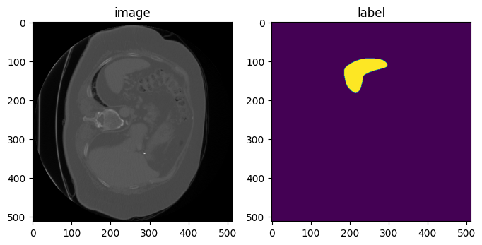
아래는 PLI를 axcodes로 적용한 것입니다.
## PLI axis ##

orientation = Orientationd(keys=["image", "label"], axcodes="PLI")
data_dict = orientation(datac_dict)
print(f"image shape: {data_dict['image'].shape}")
print(f"label shape: {data_dict['label'].shape}")
print(f"image affine after Spacing:\n{data_dict['image'].meta['affine']}")
print(f"label affine after Spacing:\n{data_dict['label'].meta['affine']}")

image, label = data_dict["image"], data_dict["label"]
plt.figure("visualise", (8, 4))
plt.subplot(1, 2, 1)
plt.title("image")
plt.imshow(image[0, :, :, 30], cmap="gray")
plt.subplot(1, 2, 2)
plt.title("label")
plt.imshow(label[0, :, :, 30])
plt.show()
image shape: (1, 512, 512, 55)
label shape: (1, 512, 512, 55)
image affine after Spacing:
tensor([[ 0.0000e+00, -9.7656e-01, 0.0000e+00, 4.7684e-07],
[-9.7656e-01, 0.0000e+00, 0.0000e+00, 4.7684e-07],
[ 0.0000e+00, 0.0000e+00, -5.0000e+00, 2.7000e+02],
[ 0.0000e+00, 0.0000e+00, 0.0000e+00, 1.0000e+00]])
label affine after Spacing:
tensor([[ 0.0000e+00, -9.7656e-01, 0.0000e+00, 4.7684e-07],
[-9.7656e-01, 0.0000e+00, 0.0000e+00, 4.7684e-07],
[ 0.0000e+00, 0.0000e+00, -5.0000e+00, 2.7000e+02],
[ 0.0000e+00, 0.0000e+00, 0.0000e+00, 1.0000e+00]])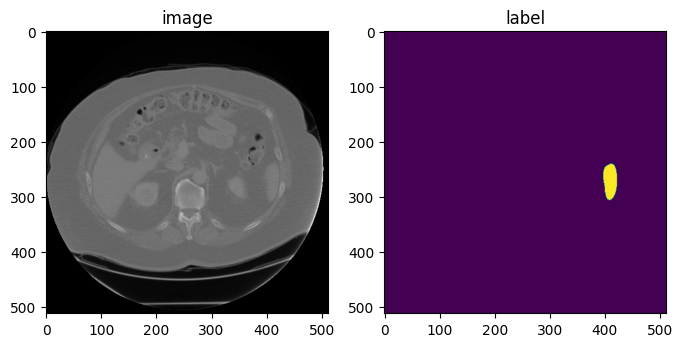
3. voxel size 통일하기
- 대부분의 input volumes들은 통일되지 않은 voxel size를 가지고 있을 가능성이 많습니다.
- 각 데이터의 NIfTI 파일에 존재하는 affine을 이용해 mm (real world) coordinate으로 변환해줄 수 있습니다.
- monai의 Spacingd는 이를 간편하게 수행할 수 있습니다.
for i in range(1,3):
    data_dict_ = loader(train_data_dicts[i])
    data_dict_ = ensure_channel_first(data_dict_)
    data_dict_ = orientation(data_dict_)
    print(f'[sample {i}]')
    print(f"image shape: {data_dict_['image'].shape}")
    print(f"label unique: {torch.unique(data_dict_['label'])}")
    print(f"image pixdim: {data_dict_['image'].pixdim}")
[sample 1]
image shape: (1, 512, 512, 168)
image shape: tensor([0., 1.])
image pixdim: tensor([0.7539, 0.7539, 1.5000], dtype=torch.float64)
[sample 2]
image shape: (1, 512, 512, 77)
image shape: tensor([0., 1.])
image pixdim: tensor([0.7422, 0.7422, 2.5000], dtype=torch.float64)- 보는바와 같이 [sample 1]과 [sample 2]의 voxel size가 다르다.
- 아래와 같이 (1,1,1) millimeter 로 맞춰 통일해주자
spacing = Spacingd(keys=["image", "label"], pixdim=(1., 1., 1.), mode=("bilinear", "nearest"))

for i in range(1,3):
    data_dict_ = loader(train_data_dicts[i])
    data_dict_ = ensure_channel_first(data_dict_)
    data_dict_ = orientation(data_dict_)
    data_dict_ = spacing(data_dict_)
    print(f'[sample {i}]')
    print(f"image shape: {data_dict_['image'].shape}")
    print(f"label unique: {torch.unique(data_dict_['label'])}")
    print(f"image pixdim: {data_dict_['image'].pixdim}")
[sample 1]
image shape: (1, 386, 386, 252)
label unique: tensor([0., 1.])
image pixdim: tensor([1., 1., 1.], dtype=torch.float64)
[sample 2]
image shape: (1, 380, 380, 191)
label unique: tensor([0., 1.])
image pixdim: tensor([1., 1., 1.], dtype=torch.float64)
4. random affine transformation
- 아래의 변환은 spatial_size로 (300, 300, 150)의 이미지 patch를 return 해준다.
- patch image는 translate_range 옵션으로 (+-40, +-40, +-20) 공간에서 랜덤하게 추출된다.
- 이미지의 center에서 translate됩니다.
- rotate_range는 x, y 축으로 (+-5) degree만큼, z축으로는 (+-45) degree 만큼 랜던하게 회전됩니다.
- random scaling은 각 축을 기준으로 +-15% 정도 랜덤하게 적용됩니다.
rand_affine = RandAffined(
    keys=["image", "label"],
    mode=("bilinear", "nearest"),
    prob=1.0,
    spatial_size=(300, 300, 150),
    translate_range=(40, 40, 20),
    rotate_range=(np.pi / 36, np.pi / 36, np.pi / 4),
    scale_range=(0.15, 0.15, 0.15),
    padding_mode="border",
)
rand_affine.set_random_state(seed=123)

affined_data_dict = rand_affine(data_dict)
print(f"image shape: {affined_data_dict['image'].shape}")

image, label = affined_data_dict["image"][0], affined_data_dict["label"][0]
plt.figure("visualise", (8, 4))
plt.subplot(1, 2, 1)
plt.title("image")
plt.imshow(image[:, :, 73], cmap="gray")
plt.subplot(1, 2, 2)
plt.title("label")
plt.imshow(label[:, :, 73])
plt.show()
image shape: (1, 300, 300, 150)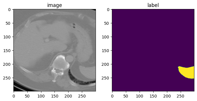
5. random elastic deformation
- 위와 비슷하게 elastic deformation의 output size도 spatial_size에 따라 결정됩니다.
- affine 변환과 elastic 변환의 조합으로 augmentation 됩니다.
- sigma_range는 deformation의 smoothness를 조절합니다. (15이상되면 CPU에 병목현상이 생길수있습니다)
- magnitude_range는 변환의 진폭(amplitude)을 조절합니다. (500 이상이면 unrealistic한 이미지가 됩니다)
rand_elastic = Rand3DElasticd(
    keys=["image", "label"],
    mode=("bilinear", "nearest"),
    prob=1.0,
    sigma_range=(5, 8),
    magnitude_range=(100, 200),
    spatial_size=(300, 300, 10),
    translate_range=(50, 50, 2),
    rotate_range=(np.pi / 36, np.pi / 36, np.pi),
    scale_range=(0.15, 0.15, 0.15),
    padding_mode="border",
)
rand_elastic.set_random_state(seed=123)

deformed_data_dict = rand_elastic(data_dict)
print(f"image shape: {deformed_data_dict['image'].shape}")

image, label = deformed_data_dict["image"][0], deformed_data_dict["label"][0]
plt.figure("visualise", (8, 4))
plt.subplot(1, 2, 1)
plt.title("image")
plt.imshow(image[:, :, 5], cmap="gray")
plt.subplot(1, 2, 2)
plt.title("label")
plt.imshow(label[:, :, 5])
plt.show()
image shape: (1, 300, 300, 10)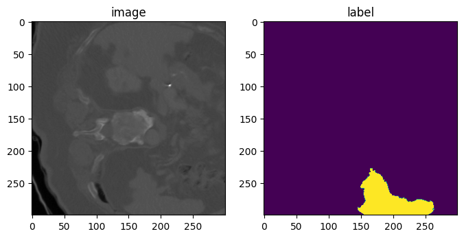
끝!
반응형
'machine learning' 카테고리의 다른 글
| [ML] 분류 평가 지표 정리(sensitivity, recall, precision, specificity, f1 score, NPV, PPV (0) | 2022.11.22 |
|---|---|
| [ML][pytorch] UNETR(21.03); UNEt TRansformers 코드 설명 및 구현 (2) | 2022.11.21 |
| [ML] ViT(20.10); Vision Transformer 코드 구현 및 설명 with pytorch (2) | 2022.11.10 |
| [ML] Dice loss & Dice Score with monai, pytorch (0) | 2022.11.08 |
| [ML][pytorch] torch.nn 과 torch.nn.Functional 의 차이 (0) | 2022.11.08 |
'machine learning' Related Articles
more


Comments